5. How PSFEx works

5.1. Overview of the software

Fig. 5.1 Global Layout of PSFEx.

The global layout of PSFEx is presented in Fig. 5.1. There are many ways to operate the software. Let us now describe the important steps in the most common usage modes.

1. PSFEx starts by examining the catalogues given in the command line. In the default operating mode, for mosaic cameras, Multi-Extension FITS (MEF) files are processed extension by extension. PSFEx pre-selects detections which are likely to be point sources, based on source characteristics such as half-light radius and ellipticity, while rejecting contaminated or saturated objects.
2. For each pre-selected detection, the “vignette” (produced by SExtractor) and a “context vector” are loaded in memory. The context vector represents the set of parameters (like position) on which the PSF model will depend explicitly.
3. The PSF modelling process is iterated 4 times. Each iteration consists of computing the PSF model, comparing the vignettes to the model reconstructed in their “local contexts”, and excluding detections that show too much departure between the data and the model.
4. Depending on the configuration, two types of Principal Component Analyses (PCAs) may be included at this stage, either to build an optimised image vector basis to represent the PSF, or to track hidden dependencies of the model. In both cases, they result in a second round of PSF modelling.
5. The PSF models are saved to disk. If requested, PSF homogenisation kernels may also be computed and written to disk at this stage. Finally, diagnostic files are generated.

5.2. Point source selection

PSFEx requires the presence of unresolved sources (stars or quasars) in the input catalogue(s) to extract a valid PSF model. In some astronomical observations, the fraction of suitable point sources that may be used as good approximations to the local PSF may be rather low. This is especially true for deep imaging in the vicinity of galaxy clusters at high galactic latitudes, where unsaturated stars may comprise only a small percentage of all detectable sources.

5.2.1. Selection criteria

To minimise as much as possible the assumptions on the shape of the PSF, PSFEx adopts the following selection criteria:

• the shape of suitable unresolved (unsaturated) sources does not depend on the flux.
• amongst image profiles of all real sources, those from unresolved sources have the smallest Full-Width at Half Maximum (FWHM).

These considerations as well as much experimentation led to adopting a first-order selection similar to the rectangular cut in the half-light-radius (\(r_{\rm h}\)) vs. magnitude plane, popular amongst members of the weak lensing community (Kaiser et al. 1995). SExtractor’s FLUX_RADIUS parameter with input parameter PHOT_FLUXFRAC \(=0.5\) provides a good estimate for \(r_{\rm h}\). In PSFEx, the “vertical” locus produced by point sources (whose shape does not depend on magnitude) is automatically framed between a minimum signal-to-noise threshold and the saturation limit on the magnitude axis, and within some margin around the local mode on the \(r_{\rm h}\) axis (Fig. 5.2). The relative width of the selection box is set by the SAMPLE_VARIABILITY configuration parameter (0.2 by default), within boundaries defined by half the SAMPLE_FWHMRANGE parameter (between 2 and 10 pixels by default). Additionally, to provide a better rejection of image artifacts and multiple objects, PSFEx excludes detections

• with a Signal-to-Noise Ratio (SNR) below the value set with the SAMPLE_MINSN configuration parameter (20 by default). The SNR is defined here as the ratio between the source flux and the source flux uncertainty.
• with SExtractor extraction FLAGS that match the mask set by the SAMPLE_FLAGMASK configuration keyword. The default mask (00fe in hexadecimal) excludes all flagged objects, except those with FLAGS = 1 (indicating a crowded environment).
• with an ellipticity exceeding the value set with the SAMPLE_MAXELLIP configuration parameter (0.3 by default). The ellipticity is defined here as \((A-B)/(A+B)\), where \(A\) and \(B\) are the lengths of the major and minor axes, respectively. The ratio \(A/B\) is also called the ELONGATION. Note that, for historical reasons, this definition differs from the one use in SExtractor, which is \((1-B/A)\)
• that include pixels that were given a weight of 0 (for weighted source extractions).

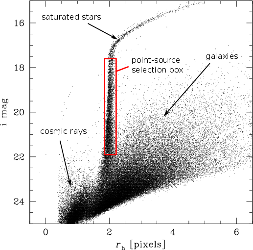
Fig. 5.2 Half-light-radius (\(r_{\rm h}\), estimated by SExtractor‘s FLUX_RADIUS) vs magnitude (MAG_AUTO) for a 520 s CFHTLS exposure at high galactic latitude taken with the Megaprime instrument in the \(i\) band. The rectangle enclosing part of the stellar locus represents the approximate boundaries set automatically by PSFEx to select point sources.

5.2.2. Iterative filtering

Despite the filtering process, a small fraction of the remaining point source candidates (typically 5-10% on ground-based optical images at high galactic latitude) is still unsuitable to serve as a realisation of the local PSF, because of contamination by neighbouring objects. Iterative procedures to subtract the contribution from neighbour stars have been successfully applied in crowded fields [6][7]. However these techniques do not solve the problem of pollution by non-stellar objects like image artifacts, a common curse of wide field imaging, and contaminated point sources still have to be filtered out.

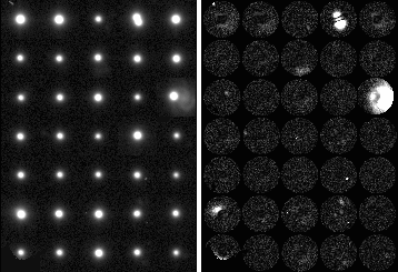
Fig. 5.3 Left: some source images selected for deriving a PSF model of a MEGACAM image (the basic rejection tests based on SExtractor flags and measurements were voluntarily bypassed to increase the fraction of contaminants in this illustration). Right: map of residuals computed as explained in the text; bright pixels betray interlopers like cosmic ray hits and close neighbour sources.

The iterative rejection process in PSFEx works by deriving a 1st-order estimate of the PSF model, and computing a map of the residuals of the fit of this model to each point source (Fig. 5.3): each pixel of the map is the square of the difference square of the model with the data, divided by the \(\sigma_i^2\) estimate from equation (3). The PSF model may be “rough” at the first iteration, hence to avoid penalising poorly fitted bright source pixels, the factor \(\alpha\) is initially set to a fairly large value, 0.1—0.3. Assuming that the fitting errors are normally distributed, and given the large number of degrees of freedom (the tabulated values of the model), the distribution of \(\sqrt{\chi^2}\) derived from the residual maps of point sources is expected to be Gaussian to a good approximation. Contaminated profiles are identified using \(\kappa\)–\(\sigma\) clipping to the distribution of \(\sqrt{\chi^2}\). Our experiments indicate that the value \(\kappa=4\) provides a consistent compromise between being too restrictive and being too permissive. PSFEx repeats the PSF modelling / source rejection process 3 more times, with decreasing \(\alpha\), before delivering the “clean” PSF model.

5.3. Modelling the PSF

In PSFEx, the PSF is modelled as a linear combination of basis vectors. Since the PSF of an optical instrument is the Fourier Transform of the auto-correlation of its pupil, the PSF of any instrument with a finite aperture is bandwidth-limited. According to the Shannon sampling theorem, the PSF can therefore be perfectly reconstructed (interpolated) from an infinite table of regularly-spaced samples. For a finite table, the reconstruction will not be perfect: extended features, such as profile wings and diffraction spikes caused by the high frequency component of the pupil function, will obviously be cropped. With this limitation in mind, one may nevertheless reconstruct with good accuracy a tabulated PSF thanks to sinc interpolation [8]. Undersampled PSFs can also be represented in the form of tabulated data provided that a finer grid satisfying Nyquist’s criterion is used [9][10].

For reasons of flexibility and interoperability with other software, we chose to represent PSFs in PSFEx as small images with adjustable resolution. These PSF “images” can be either derived directly, treating each pixel as a free parameter (“pixel” vector basis), or more generally as a combination of basis vector images.

5.3.1. Pixel basis

The pixel basis is selected by setting BASIS_TYPE to PIXEL.

Recovering aliased PSFs - If the data are undersampled, unaliased Fourier components can in principle be recovered from the images of several point sources randomly located with respect to the pixel grid, using the principle of super-resolution [11]. Working in the Fourier domain, [12] shows how PSFs from the Hubble Space Telescope Planetary Camera and Wide-Field Planetary Camera can be reconstructed at 3 times the original instrumental sampling from a large number of undersampled star images. However, solving in the Fourier domain gives far from satisfactory results with real data. Images have boundaries; the wings of point source profiles may be contaminated with artifacts or background sources; the noise process is far from stationary behind point sources with high S/N, because of the local photon-noise contribution from the sources themselves. All these features generate spurious Fourier modes in the solution, which appear as parasitic ripples in the final, super-resolved PSF.

A more robust solution is to work directly in pixel space, using an interpolation function; we may use the same interpolation function later on to fit the tabulated PSF model for point source photometry. Let \(\boldsymbol{\phi}\) be the vector representing the tabulated PSF, \(h_s(\boldsymbol{x})\) an interpolation function, \(\eta\) the ratio of the PSF sampling step to the original image sampling step (oversampling factor). The interpolated value at image pixel \(i\) of \(\boldsymbol{\phi}\) centered on coordinates \(\boldsymbol{x}_s\) is

(1)\[ \phi_{i}'(\boldsymbol{x}_s) = \sum_j h_s\left(\boldsymbol{x}_j - \eta\,(\boldsymbol{x}_i - \boldsymbol{x}_s)\right)\phi_j\]

Note that \(\eta\) can be less than 1 in the case where the PSF is oversampled. Using multiple point sources \(s\) sharing the same PSF, but centred on various coordinates \(\boldsymbol{x}_s\), and neglecting the correlation of noise between pixels, we can derive the components of \(\boldsymbol{\phi}\) that provide the best fit (in the least-square sense) to the point source images by minimising the cost function:

(2)\[ E(\boldsymbol{\phi}) = \chi^2(\boldsymbol{\phi}) = \sum_s \sum_{i \in {\cal D}_s} \frac{\left(p_{i} - f_s \phi_{i}'(\boldsymbol{x}_s)\right)^2}{\sigma_{i}^2},\]

where \(f_s\) is the integrated flux of point source \(s\), \(p_i\) the pixel intensity (number of counts in ADUs) recorded above the background at image pixel \(i\), and \({\cal D}_s\) the set of pixels around \(s\). In the variance estimate of pixel \(i\), \(\sigma_{i}^2\), we identify three contributions:

(3)\[ \sigma_{i}^2 = \sigma_{\rm b}^2 + \frac{p_i}{g} + (\alpha\,p_i)^2 \ ,\]

where \(\sigma_{\rm b}^2\) is the pixel variance of the local background, \(p_i/g\), where \(g\) is the detector gain in \(e^-\)/ADU (which must have been set appropriately before running SExtractor, is the variance contributed by photons from the source itself. The third term in equation (3) will generally be negligible except for high \(p_i\) values; the \(\alpha\) factor accounts for pixel-to-pixel uncertainties in the flat-fielding, variation of the intra-pixel response function, and apparent fluctuations of the PSF due to interleaved “micro-dithered” observations [1] or lossy image resampling. The value of \(\alpha\) is set by user with the PSF_ACCURACY configuration parameter. Depending on image quality, suitable values for PSF_ACCURACY range from less than one thousandth to 0.1 or even more. The default value, 0.01, should be appropriate for typical CCD images.

The flux \(f_s\) is measured by integrating over a defined aperture, which defines the normalisation of the PSF. Its diameter must be sufficiently large to prevent the measurement from being too sensitive to centering or pixelisation effects, but not excessively large to avoid too strong S/N degradation and contamination by neighbours. In practice, a \(\approx 5''\) diameter provides a fair compromise with good seeing images (PSF FWHM \(< 1.2''\)), but smaller in very crowded fields.

Interpolating the PSF model - As we saw, one of the main interests of interpolating the PSF model in direct space is that it involves only a limited number of PSF “pixels”. However, as in any image resampling task, a compromise must be found between the perfect Shannon interpolant (unbounded sinc function), and simple schemes with excessive smoothing and/or aliasing properties like bi-linear interpolation (“tent” function) [13]. Experimenting with the SWarp image resampling prototype [14], we found that the Lanczos4 interpolant

(4)\[\begin{split} h(x) = \left\{ \begin{array}{ll} 1 & x=0 \\ \hbox{sinc}(x)\,\hbox{sinc} \left ({x/4}\right) & 0 < |x|\leq 4 \\ 0 & |x| > 4 \end{array} \right. \ ,\end{split}\]

where \(\hbox{sinc}(x) = \sin(\pi x)/(\pi x)\)[2], provides reasonable compromise: the kernel footprint is 8 PSF pixels in each dimension, and the modulation transfer function is close to flat up to \(\approx 60\%\) of the Nyquist frequency (Fig. 5.4). A typical minimum of 2 to 2.5 pixels per PSF FWHM is required to sample an astronomical image without generating significant aliasing [15]. Consequently, an appropriate sampling step for the PSF model would be \(1/4^{\rm th}\) of the PSF FWHM. This is automatically done in PSFEx, when the PSF_SAMPLING configuration parameter is set to 0 (the default). The PSF sampling step may be manually adjusted (in units of image pixels) by simply setting PSF_SAMPLING to a non-zero value.

Fig. 5.4 The Lanczos4 interpolant in one dimension (left), and its modulation transfer function (right).

Regularisation - For \(\eta\gg 1\), the system of equations obtained by minimising equation (2) becomes ill-conditioned and requires regularisation [16]. Our experience with PSFEx shows that the solutions obtained over the domain of interest for astronomical imaging (\(\eta \le 3\)) are robust in practice, and that regularisation is generally not needed. However, it may happen, especially with infrared detectors, that samples of undersampled point sources are contaminated by image artifacts; and solutions computed with equation (2) become unstable. We therefore added a simple Tikhonov regularisation scheme to the cost function:

(5)\[ E(\boldsymbol{\phi}) = \chi^2(\boldsymbol{\phi}) + \Arrowvert \textbf{T} \boldsymbol{\phi}\Arrowvert^2.\]

In image processing problems the (linear) Tikhonov operator \(\mathrm{T}\) is usually chosen to be a high-pass filter to favour “smooth” solutions. PSFEx adopts a slightly different approach by reducing \(\mathrm{T}\) to a scalar weight \(1/\sigma_{\phi}^2\) and performing a procedure in two steps.

1. PSFEx makes a first rough estimate of the PSF by simply shifting point sources to a common grid and computing a median image \(\boldsymbol{\phi}^{(0)}\). With undersampled data this image represents a smooth version of the real PSF.
2. Instead of fitting directly the model to pixel values, PSFEx fits the difference \(\Delta\boldsymbol{\phi}\) between the model and \(\boldsymbol{\phi}^{(0)}\). \(E(\boldsymbol{\phi})\) becomes

(6)\[ E(\boldsymbol{\phi}) = \sum_s \sum_{i \in {\cal D}_s} \frac{\left[p_{i} - f_s \left(\phi_{i}'^{(0)}(\boldsymbol{x}_s) +\Delta\phi_{i}'(\boldsymbol{x}_s)\right)\right]^2}{\sigma_{i}^2} + \sum_j \frac{\Delta\phi_j^2}{\sigma_{\phi}^2}.\]

Minimising equation (6) with respect to the \(\Delta\phi_j\)’s comes down to solving the system of equations

(7)\[\begin{split}\begin{aligned} 0 & = &\frac{\partial E}{\partial \Delta\phi_k}\nonumber\\ &= & 2\,f_s \sum_s \sum_{i \in {\cal D}_s} \frac{1}{\sigma_{i}^2} h_s\left(\boldsymbol{x}_k - \eta\,[\boldsymbol{x}_i - \boldsymbol{x}_s]\right)\nonumber\\ && \times \left(f_s \sum_j h_s\left(\boldsymbol{x}_j - \eta\,[\boldsymbol{x}_i - \boldsymbol{x}_s]\right)(\phi_j^{(0)} + \Delta\phi_j) - p_{i}\right)\nonumber\\ && + \frac{2}{\sigma_{\phi}^2}\, \Delta\phi_k \ .\end{aligned}\end{split}\]

In practice the solution appears to be fairly insensitive to the exact value of \(\sigma_{\phi}\) except with low signal-to-noise conditions or contamination by artifacts. \(\sigma_{\phi}\approx 10^{-2}\) seems to provide a good compromise by bringing efficient control of noisy cases but no detectable smoothing of PSFs with good data and high signal-to-noise.

The system in equation (7) is solved by PSFEx in a single pass. Much of the processing time is actually spent in filling the normal equation matrix, which would be prohibitive for large PSFs if the sparsity of the design matrix were not put to contribution to speed up computations.

5.3.2. Gauss-Laguerre basis

The pixel basis is quite a “natural” basis for describing in tabulated form bandwidth-limited PSFs with arbitrary shapes. But in a majority of cases, more restrictive assumptions can be made about the PSF that allow the model to be represented with a smaller number of components, e.g. a bell-shaped profile, a narrow scale range... Less basis vectors make for more robust models. For close-to-Gaussian PSFs, the Gauss-Laguerre basis is a sensible choice.

The Gauss-Laguerre basis is selected by setting BASIS_TYPE to be GAUSS-LAGUERRE. The Gauss-Laguerre functions, also known as polar shapelets in the weak-lensing community [4] provide a “natural” orthonormal basis for broadly Gaussian profiles:

\[\!\psi_{n,m}(r,\theta) = \frac{(-1)^{(n-|m|)/2}}{\sqrt\pi\,\sigma} \sqrt{\frac{[(n\!-\!|m|)/2]!}{[(n\!+\!|m|)/2]!}} \left(\frac{r}{\sigma}\right)^{|m|} \exp\left[-\frac{1}{2}\left(\frac{r}{\sigma}\right)^2 \!-\! i m\theta\right] L^{|m|}_{(n\!-\!|m|)/2}\left(\frac{r^2}{\sigma^2}\right) ,\]

where \(\sigma\) is a typical scale for \(r\), \((n-|m|)/2 \in \mathbb{N}\) and \(L^{k}_n(x)\) is the associated Laguerre polynomial

\[\begin{split}\begin{aligned} L^{k}_n(x) & = & \frac{1}{n!}\,x^{-k}\,{\rm e}^x\, \frac{{\rm d}^n}{{\rm d}x^n}\left(x^{n+k}e^{-x}\right)\\ & = & \sum_{j=0}^n\frac{(k+n)!}{j!\,(n-j)!\,(j+k)!}\,(-x)^j. \end{aligned}\end{split}\]

The number of shapelet vectors with \(n \le n_{\rm max}\) is

\[N_{\rm max} = {(n_{\rm max}+1)\,(n_{\rm max}+2)\over 2} \ .\]

Shapelet decompositions with finite \(n \le n_{\rm max}\) are only able to probe a restricted range of scales. [17] quotes \(r_{\rm min} = \sigma /\sqrt{n_{\rm max}+1}\) and \(r_{\rm max} = \sigma\sqrt{n_{\rm max}+1}\) as the standard deviation of the central lobe and the whole shapelet profile, respectively (so that \(\sigma\) is the geometric mean of \(r_{\rm min}\) and \(r_{\rm max}\)). In practice, the diameter of the circle enclosing the region where images can be fitted with shapelets is only about \(\approx 2.5\, r_{\rm max}\). Hence modelling accurately both the wings and the core of PSFs with a unique set of shapelets requires a very large number of shapelet vectors, typically several hundreds.

Fig. 5.5 Left: part of a simulated star field image with strong undersampling. Right, from top to bottom: (a) simulated optical PSF, (b) simulated PSF convolved by the pixel response, (c) PSF recovered by PSFEx at 4.5 times the image resolution from a random sample of 212 stars extracted in the simulated field above, using the “pixel” vector basis, and (d) PSF recovered using the “shapelet” basis with \(n_{\rm max} = 16\).

5.3.3. Other bases

With the BASIS_TYPE FILE option, PSFEx offers the possibility to use an external image vector basis. The basis should be provided as a FITS datacube (the \(3^{\rm rd}\) dimension being the vector index), and the file name given to PSFEx with the BASIS_NAME parameter. External bases do not need to be normalised.

5.4. Managing PSF variations

Few imaging systems have a perfectly stable PSF, be it in time or position: for most instruments the approximation of a constant PSF is valid only on a small portion of an image at a time. Position-dependent variations of the PSF on the focal plane are generally caused by optics, and exhibit a smooth behaviour which can be modelled with a low-order polynomial.

The most intuitive way to generate variations of the PSF model is to apply some warping to it (enlargement, elongation, skewness, ...). But this description is not appropriate with PSFEx because of the non-linear dependency of PSF vector components towards warping parameters. Instead, one can extend the formalism of equation (6) by describing the PSF as a variable, linear combination of PSF vectors \(\boldsymbol{\phi}_c\); each of them associated to a basis function \(X_c\) of some parameter vector \(\boldsymbol{p}\) like image coordinates:

(8)\[ E(\boldsymbol{\phi}) = \sum_s \sum_{i \in {\cal D}_s} \frac{\left(p_{i} - f_s \sum_c X_c(\boldsymbol{p}) \left(\phi_{c\,i}'^{(0)}(\boldsymbol{x}_s) +\Delta\phi_{c\,i}'(\boldsymbol{x}_s)\right)\right)^2}{\sigma_{i}^2} + \sum_j \sum_c \frac{\Delta\phi_{c\,j}^2}{\sigma_{\phi}^2} \ .\]

The basis functions \(X_c\) in the current version of PSFEx are limited to simple polynomials of the components of \(\boldsymbol{p}\). Each of these components \(p_l\) belongs to a “PSF variability group” \(g =0,1,...,N_g\), such that

(9)\[ X_c(\boldsymbol{p}) = \prod_{g\le N_g} \left( \prod_{(\sum_{l \in \Lambda_g} d_l)\le D_g}p_{l}^{d_{l}}\right),\]

where \(\Lambda_g\) is the set of \({l}\)’s that belongs to the distortion group \(g\), and \(D_{g} \in \mathbb{N}\) is the polynomial degree of group \(g\). The polynomial engine of PSFEx is the same as the one implemented in the SCAMP software [18] and can use any set of SExtractor and/or FITS header parameters as components of \(p\). Although PSF variations are more likely to depend essentially on source position on the focal plane, it is thus possible to include explicit dependency on parameters such as telescope position, time, source flux (Fig. 5.7) or instrument temperature.

The \(p_l\) components are selected using the PSFVAR_KEYS configuration parameter. The arguments can be names of SExtractor measurements, or keywords from the image FITS header representing numerical values. FITS header keywords must be preceded with a colon (:), like in :AIRMASS. The default PSFVAR_KEYS are X_IMAGE,Y_IMAGE.

The PSFVAR_GROUPS configuration parameters must be filled in in combination with the PSFVAR_KEYS to indicate to which PSF variability group each component of \(\boldsymbol{p}\) belongs. The default for PSFVAR_GROUPS is 1,1, meaning that both PSFVAR_KEYS belong to the same unique PSF variability group. The polynomial degrees \(D_{g}\) are set with PSFVAR_DEGREES. The default PSFVAR_DEGREES is 2. In practice, a third-degree polynomial on pixel coordinates (represented by 20 PSF vectors) should be able to map PSF variations with good accuracy on most exposures (Fig. 5.6).

Fig. 5.6 Example of PSF mapping as a function of pixel coordinates in PSFEx. Left: PSF component vectors for each polynomial term derived from the CFHTLS-deep “D4” \(r\)-band stack observed with the MEGACAM camera. A third-degree polynomial was chosen for this example. Note the prominent variation of PSF width with the square of the distance to the field centre. Right: reconstruction of the PSF over the \(1^\circ\) field of view (the grey scale has been slightly compressed to improve clarity).

Fig. 5.7 Example of PSF mapping on images from a non-linear imaging device. 1670 point sources from the central \(4096\times4096\) pixels of a photographic scan (SERC J #418 survey plate, courtesy of J. Guibert, CAI, Paris observatory) were extracted using SExtractor, and their images run through PSFEx. A sample is shown at the top-left. The PSF model was given a \(6^{\rm th}\) degree polynomial dependency on the instrumental magnitude measured by SExtractor (MAG_AUTO). Middle: PSF components derived by PSFEx. Bottom: reconstructed PSF images as a function of decreasing magnitude. Top-right: sample residuals after subtraction of the PSF-model.

5.5. Quality assessment

Maintaining a certain level of image quality, and especially PSF quality, by identifying and rejecting “bad” exposures, is a critical issue in large imaging surveys. Image control must be automated, not only because of the sheer quantity of data in modern digital surveys, but also to ensure an adequate level of consistency. Automated PSF quality assessment is traditionally based upon point source FWHM and ellipticity measurements. Although this is certainly efficient for finding fuzzy or elongated images, it cannot make the distinction between e.g. a defocused image and a moderately bad seeing.

PSFEx can trace out the apparition of specific patterns using customized basis functions. Moreover, PSFEx implements a series of generic quality measurements performed on the PSF model as it varies across the field of view. The main set of measurements is done in PSF pixel space (with oversampling factor \(\eta\)) by comparing the actual PSF model vector \(\boldsymbol{\phi}\) with a reference PSF model \(\rho(\boldsymbol{x}')\). We adopt as a reference model the elliptical Moffat function [2] that fits best (in the chi-square sense) the model (10):

(10)\[ \rho(\boldsymbol{x}') = I_0 \left(1 + \left|\left|\mathrm{A}(\boldsymbol{x}'-\boldsymbol{x}'_c)\right|\right|^2\right)^{-\beta},\]

with

\[\begin{split}\mathrm{A} = \frac{4}{\eta}\,(2^{-\frac{1}{\beta}} - 1) \left(\begin{array}{lr} \ \ \ \cos \theta / W_{\rm max}\ & \ \sin \theta / W_{\rm max}\\ -\sin \theta / W_{\rm min}\ & \ \cos \theta / W_{\rm min}\\ \end{array}\right),\end{split}\]

where \(I_0\) is the central intensity of the PSF, \(\boldsymbol{x}'_c\) the central coordinates (in PSF pixels), \(W_{\rm max}\), the PSF FWHM along the major axis, \(W_{\rm min}\) the FWHM along the minor axis, and \(\theta\) the position angle (6 free parameters). As a matter of fact, the Moffat function provides a good fit to seeing-limited images of point-sources, and to a lesser degree, to the core of diffraction-limited images for instruments with circular apertures [19]: in most imaging surveys, the “correct” instrumental PSF will be very similar to a Moffat function with low ellipticity.

Since PSFEx is meant to deal with significantly undersampled PSFs, another fit — which we call “pixel-free” — is also performed, where the Moffat model is convolved with a square top-hat function the width of a physical pixel, as an approximation to the real intra-pixel response function. The width of the pixel is set to 1 in image sampling step units by default, which corresponds to a 100% fill-factor. It can be changed using the PSF_PIXELSIZE configuration parameter. Future versions of PSFEx might propose more sophisticated models of the intra-pixel response function.

The (non-linear) fits are performed using the LevMar implementation of the Levenberg-Marquardt algorithm [20]. They are repeated at regular intervals on a grid of PSF parameter vectors \(\boldsymbol{p}\), generally composed of the image coordinates \(\boldsymbol{x}\)), but with possible additional parameters such as time, observing conditions, etc. The density of the grid may be adjusted using the PSFVAR_NSNAP configuration parameter. The default value for PSFVAR_NSNAP is 9 (snapshots per component of \(\boldsymbol{p}\)). Larger numbers can be useful to track PSF variations on large images with greater accuracy; but beware of the computing time, which increases as the total number of PSF snapshots (grid points).

The average FWHM \((W_{\rm max}+W_{\rm min})/2\), ellipticity \((W_{\rm max}-W_{\rm min})/(W_{\rm max}+W_{\rm min})\) and \(\beta\) parameters derived from the fits provide a first set of local IQ estimators (Fig. 5.8). The second set is composed of the so-called residuals index

(11)\[ r = 2 \frac{\sum_i \left(\phi_i+\rho'(\boldsymbol{x}'_i)\right) \left|\phi_i-\rho'(\boldsymbol{x}'_i)\right|} {\sum_i \left(\phi_i+\rho'(\boldsymbol{x}'_i)\right)^2}\]

and the asymmetry index

(12)\[ \alpha = 2 \frac{\sum_i \left(\phi_i+\phi_{N-i}\right) \left|\phi_i-\phi_{N-i}\right|} {\sum_i \left(\phi_i+\phi_{N-i}\right)^2},\]

where the \(\phi_{N-i}\)’s are the point-symmetric counterparts to the \(\phi_i\) components.

Fig. 5.8 FWHM map (left) and ellipticity map (right) generated by PSFEx from a CFHTLS-Wide exposure. The maps and the individual Megaprime CCD footprints on the sky are presented in gnomonic projection (north on top, east at left). PSF variations are modelled independently on each CCD using a \(3^{\rm rd}\) degree polynomial (see text).

[1]

Micro-dithering consists of observing \(n^2\) times the same field with repeated \(1/n\) pixel shifts in each direction to provide properly sampled images despite using large pixels. Although the observed frames can in principle be recombined with an interleaving reconstruction procedure, changes in image quality from exposure to exposure may often lead to jaggies (artifacts) along gradients of source profiles, as can sometimes be noticed in DeNIS or WFCAM images.

[2]	This is the definition of the normalised sinc function, which should not be confused with the un-normalised definition of \(\hbox{sinc}(x) = \sin(x)/x\).